Multiple Simulated Annealing with Range Limitation
- Informations
- Introduction
- Related Work
- Method : Range Limitation
-
Experiments
- Table 1. Benchmark of various simulated annealing algorithm.
- Table 2. Mean score benchmark of multiple simulated annealing range limitation algorithm with various coefficients. The horizontal axis is the number of range limitation and the vertical axis is the number of agent.
- Table 3. Best score benchmark of multiple simulated annealing range limitation algorithm with various coefficients. The horizontal axis is the number of range limitation and the vertical axis is the number of agent.
Informations
- Project GitHub Repository
- Report
- Date : 2024.05
- Writter : 9tailwolf
- This project is for the KAIST 2024 Spring IE437 class assignment.
Introduction
This method is to find the argument that can maximize object value from a block box function. I tried some method based on Simulated Annealing. Simulated Annealing is an approximate method to solve an optimization problem and is used in situations where finding solution is computationally expensive or realistically difficult. This method is inspired by the annealing process in metallurgy, the process of heating a material and then slowly cooling it to create a stable crystal structure.
Related Work
Simulated Annealing
Simulated Annealing is used to optimize the objective function $f(x)$. where $x$ represents the value in the solution space. The goal is to find the value of $x$ that maximize $f(x)$. The algorithm follows below steps.
-
Step 0 : Simulated annealing start with temperature $T \Leftarrow T_{0}$ and Initial random solution $x \in [d]$, $d$ is the dimension of input(i.e. in our assignment 2 problem, $d = 5$). Temperature is used during the exploration process to decide whether to continue the search or find a new path, and it changes in each process.
-
Step 1 : In the existing solution $x$, the nearest neighbor solution $x’ \Leftarrow x + \delta $ is randomly selected.
-
Step 2 : Calculate $\alpha \Leftarrow f(x’) - f(x)$.
-
Step 3 : If $\alpha > 0$, then substitute the existing solution as a neighboring solution $x \Leftarrow x’$ and return to Step 1. Otherwise, Randomly re-initialize the solution $x$ with the probability $e^\frac{-\alpha}{T}$. Finally, Change the temperature according to the cooling rule by $T \Leftarrow Cooling(T)$.
-
Step 4 : When enough solutions are obtained or the temperature has dropped sufficiently, the algorithm done.
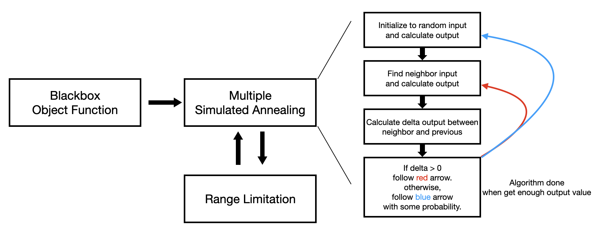
Simulated Annealing : Multiple Simulated Annealing
Multiple Simulated Annealing is a traditional method that finds the optimal solution while multiple agents share their information. I applied an algorithm that applies simulated annealing through the highest optimal solution of all multiple agents. Through this method, agents that are far from the solution can be quickly initialized and the optimal solution can be found more quickly.
The algorithm only needs small change from the simulated annealing above.
-
Step 0 : Same as Simulated Annealing Step 0. But the Initial solution is $X \in [d \times n]$, where $d$ is the dimension of input and $n$ is the number of agent. Moreover, global optimal value initialize by $f_{optimal} \Leftarrow 0$.
-
Step 1 : Same as simulated annealing Step 1. In the existing solution $x$, the nearest neighbor solution $x’ = x + \delta $ is randomly selected.
-
Step 2 : Calculate $\alpha \Leftarrow f(x’) - f_{optimal}$.
-
Step 3 : Same as simulated annealing Step 3, but assign $f_{optimal} \Leftarrow f(x’)$ when $\alpha > 0$.
-
Step 4 : Same as simulated annealing Step 4. When enough solutions are obtained or the temperature has dropped sufficiently, the algorithm done.
Method : Range Limitation
Range limitation is the newly suggested method in this algorithm. This is a method to apply multiple search more effectively and explores more deeply the midpoint of the solution of the agent with the highest score. The boundary is gradually reduced so that useless input ranges can be removed. Since it is difficult to find a global optimal value at the beginning of the algorithm, the range limitation only applies a little at the beginning, but becomes more significant towards the end.
-
Step 0 : Initialize $X \in [d \times n]$ to random value, with range $R = [d \times 2]$. $d$ is the input dimension, and the $n$ is the number of agent. And similarly to multiple simulated annealing, global optimal value initialize by $f_{optimal} \Leftarrow 0$.
-
Step 1 : Same as simulated annealing Step 1. In the existing solution $x$, the nearest neighbor solution $ x’ \Leftarrow x + \delta $ is randomly selected. But $x_{i}’$ that satisfy $ R_{i0} \leq x_{i}’ \leq R_{i1}$ for all $i$.
-
Step 2 : Same as simulated annealing Step 2. Calculate $\alpha \Leftarrow f(x’) - f_{optimal}$.
-
Step 3 : Same as simulated annealing Step 3.
-
Step 4 : When enough solutions are obtained or the temperature has dropped sufficiently, $R \Leftarrow R / r$, where $r = l(i)$, $l$ is the $R \Rightarrow R$ function which return the range limitation value, $i$ is the number of iteration. Function $l$ is more greater when $i$ is more greater. And come back to Step 1 with newly initialized $x$ that satisfy $R_{i0} \leq x_{i} \leq R_{i1}$ for all $i$.
-
Step 5 : When algorithm get enough solution, then algorithm done.
Experiments
I experimented some block box function with five inputs-one output. Below is the result of my experiments
| Object | SA | MSA | SA+RL | MSA+RL |
|---|---|---|---|---|
| $\text{NN+BN}_{mean}$ | 78.640 | 90.718 | 78.595 | 90.900 |
| $\text{NN+BN}_{best}$ | 87.521 | 90.838 | 82.852 | 90.914 |
| $\text{SVR}_{mean}$ | 79.661 | 86.146 | 80.604 | 86.153 |
| $\text{SVR}_{best}$ | 86.142 | 86.152 | 83.729 | 86.153 |
Table 1. Benchmark of various simulated annealing algorithm.
The experiments show that the \textbf{MSA+RL} method worked effectively compared to the existing simulated annealing. Additionally, I could see that existing SA and MSA were working well. But the SA+RL shows bad performance.
Below is the mean score benchmark of multiple simulated annealing range limitation algorithm with various coefficients. The horizontal axis is the number of range limitation and the vertical axis is the number of agent.
| Agent| RL | 10 | 30 | 50 | 100 | 200 |
|---|---|---|---|---|---|
| $10_{mean}$ | 88.456 | 88.117 | 88.716 | 89.170 | 89.273 |
| $30_{mean}$ | 89.041 | 89.342 | 89.357 | 89.395 | 89.399 |
| $50_{mean}$ | 89.125 | 89.323 | 89.360 | 89.402 | 89.405 |
| $100_{mean}$ | 89.319 | 89.383 | 89.407 | 89.407 | 89.410 |
| $200_{mean}$ | 89.354 | 89.395 | 89.410 | 89.410 | 89.413 |
Table 2. Mean score benchmark of multiple simulated annealing range limitation algorithm with various coefficients. The horizontal axis is the number of range limitation and the vertical axis is the number of agent.
Below is the best score benchmark of multiple simulated annealing range limitation algorithm with various coefficients. The horizontal axis is the number of range limitation and the vertical axis is the number of agent.
| Agent| RL | 10 | 30 | 50 | 100 | 200 |
|---|---|---|---|---|---|
| $10_{best}$ | 89.147 | 89.371 | 89.386 | 89.395 | 89.408 |
| $30_{best}$ | 89.319 | 89.414 | 89.411 | 89.411 | 89.413 |
| $50_{best}$ | 89.394 | 89.401 | 89.408 | 89.413 | 89.413 |
| $100_{best}$ | 89.398 | 89.411 | 89.416 | 89.415 | 89.413 |
| $200_{best}$ | 89.411 | 89.411 | 89.413 | 89.416 | 89.416 |
Table 3. Best score benchmark of multiple simulated annealing range limitation algorithm with various coefficients. The horizontal axis is the number of range limitation and the vertical axis is the number of agent.
The result shows when the number of agents and range limitations exceeds a certain level, The optimal solution could be found. In most cases, the optimal value was found, but on average, the number of cases that were closest to the optimal solution increased as the number of agents and range limitations increased.