How Can Find Ideal Racing Line? - Dynamic Programming
Simulation, Optimization
- Project GitHub Repository : HERE
- Date : 2023.11.27 ~ 2023.12.12
- Writter : 9tailwolf
Project Overview
Every track of circuit has a optimal racing line. It is not only depended on each cars, but also by track conditions. In this project, I apply real-physics based optimization algorithm for finding racing line.
Algorithm
Dynamic programming
Dynamic Programming is a useful algorithm for several optimal problem because it can reduce duplicated computation by saving some datas. It assume that optimal state $S(t)$ can find by $S(t) = f(S(t’)) (t’ < t) $.
In Circuit, tracks are seperated of each states. As shown in the above figure, there is a way to go from the previous state to the next state. States are determined by distance.
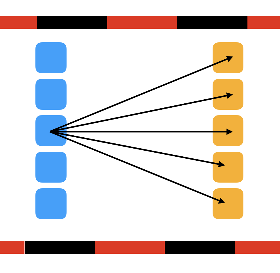
I made some nodes for each states. It represented position. There is a lot of way to go next state in each previous positions. Positions of the same state are separated by the same distance and it is perpendicular to the direction of travel.
There is another condition too. Not only location but also speed are factors that can vary. State movement must be optimized considering the initial and final speeds.
Below is a all condition of each state.
- Initial Position
- Final Position
- Initial Velocity
- Final Velocity
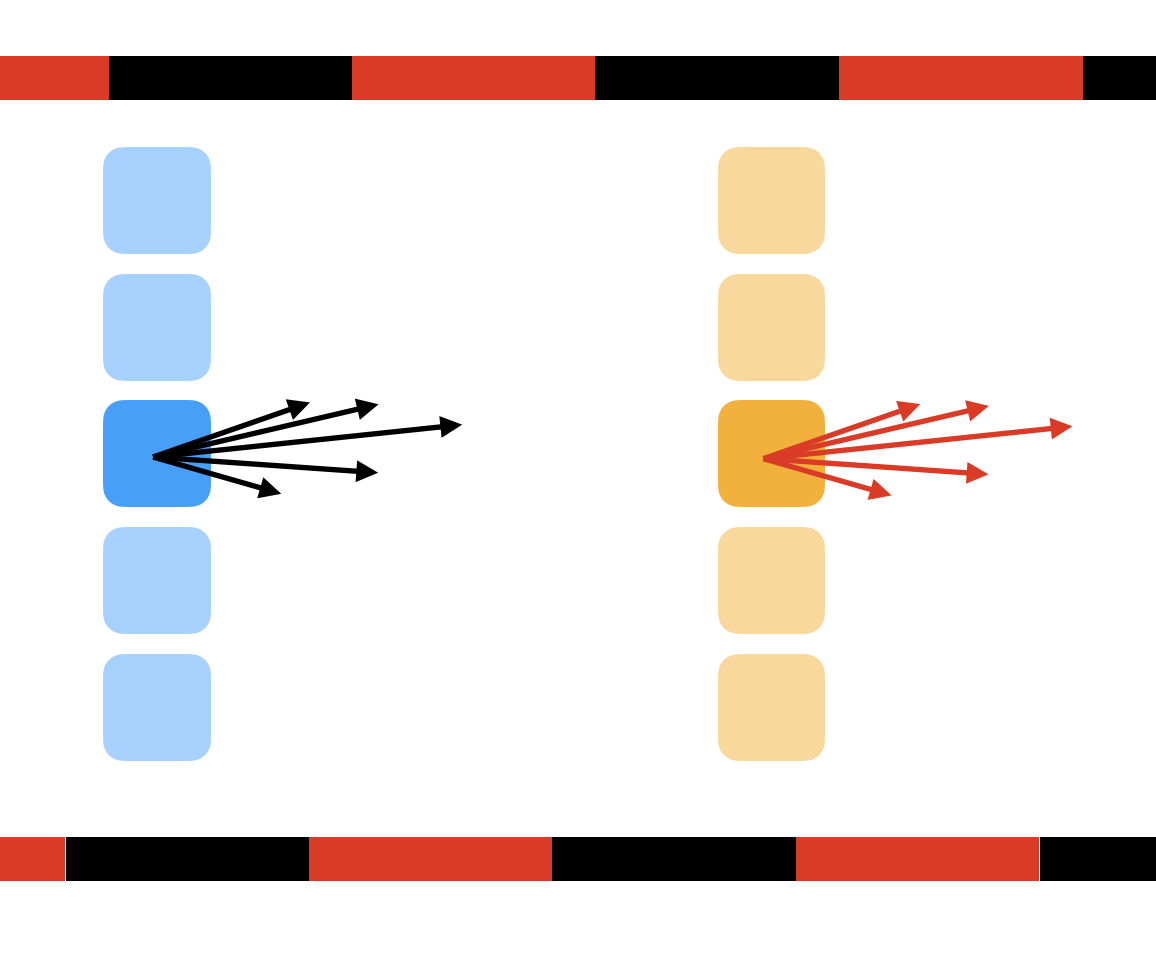
Therefore, the best state can be represented by
$S(t, \vec{p_{1}}, \vec{v_{1}}) = min{S(t-1, \vec{p_{2}}, \vec{v_{2}})}$
which $\vec{p_{1}}$ is final position, $\vec{v_{1}}$ is final velocity, $\vec{p_{2}}$ is initial position, $\vec{v_{2}}$ is initial velocity.
In other words, there are various angles and speed methods for the position of each state.
The below code is the overall process of dynamic programming. It can reduce computation $O((n^{2}m^{2}l^{2})^{k})$ to $O(k^{2}n^{2}m^{2}l^{2})$
for i in range(1,self.length):
    for node in range(self.node_size): # current position
        for v in range(self.velocity_interval): # current speed
            for t in range(self.theta_interval): # current theta
                for pre_node in range(self.node_size): # previous position
                    for pre_v in range(self.velocity_interval): # previous speed
                        for pre_t in range(self.theta_interval): # previous theta
                            if if dp[i-1][pre_node][pre_v][pre_t] != math.inf:
                                pass
                            if dp[i][node][v][t] > dp[i-1][pre_node][pre_v][pre_t] + self.cost(i,node,v,t,i-1,pre_node,pre_v,pre_t):
                                selected[i][node][v][t] = (pre_node,pre_v,pre_t)
                                dp[i][node][v][t] = dp[i-1][pre_node][pre_v][pre_t] + self.cost(i,node,v,t,i-1,pre_node,pre_v,pre_t)
Physics Limitation
- Angles Limitation
In motion, changes of position and direction of speed must be similar. Velocity can suppose as average of initial velocity and final velocity. Therefore,
$\angle (\vec{p_{1}} - \vec{p_{2}}) \approx \angle (\vec{v_{1}} + \vec{v_2})$
- Centripetal Force Limitation
When car moves in a circle, there is a limitation depends on velocity. It is because centripetal force has a limitation. Centripetal force is proportional to centripetal accelation, which is $\frac{v^{2}}{r}$.
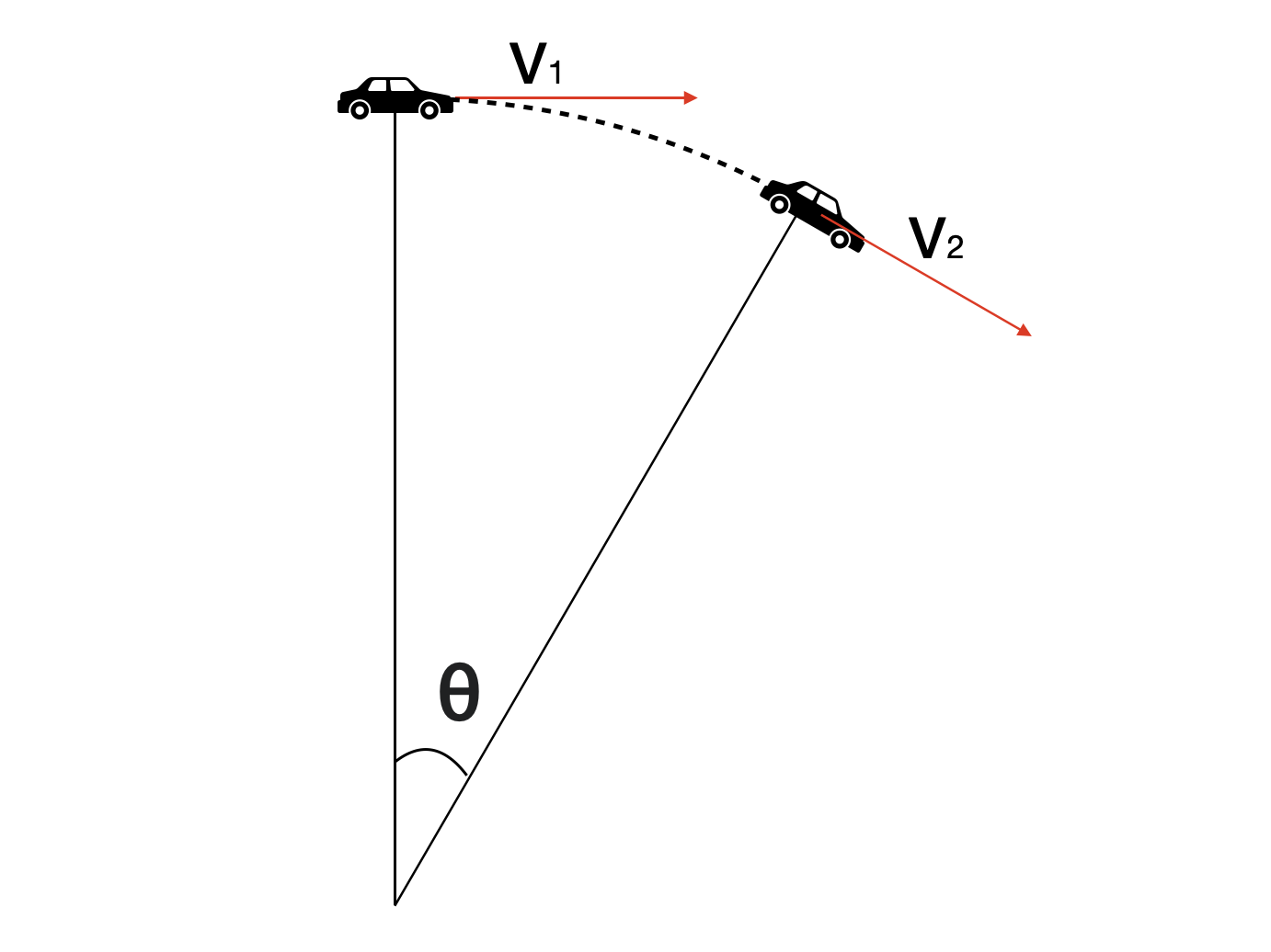
Square of speed is $\vec{v}^{2} = \left| (\vec{v_{1}}+\vec{v_{2}}) \right|^{2}$, and radius is $r = \frac{dl}{\theta} \approx \frac{ds}{\theta} = \frac{ds}{\angle v_{1} v_{2}}$.
Therefore, $ \frac{\left| (\vec{v_{1}}+\vec{v_{2}}) \right|^{2} \left| (\vec{p_{1}} - \vec{p_{2}}) \right|}{\angle v_{1} v_{2}} < a$, which $a$ is limitation of centripetal force.
- Accelation Limitation
When accelerating, rotating movements are very difficult. Therefore, when accelerating, $\angle (\vec{p_{1}} - \vec{p_{2}}) \approx \angle (\vec{v_{1}} + \vec{v_2})$ more elaborately.
When every conditions are not violate limitation, then compuate time by using below formula. $t = \frac{\left| \vec{p_{1}} - \vec{p_{2}} \right|}{\left| \vec{v_{1}} + \vec{v_2} \right|}$
The below code is the overall process of physics limitation.
def get_velocity(self,i):
    if i<0 or i>= self.velocity_interval:
        raise 'Velocity Error'

    return (i) * (self.max_velocity-self.min_velocity) / (self.velocity_interval-1) + self.min_velocity

def get_theta(self,i):
    if i<0 or i>= self.theta_interval:
        raise 'Theta Error'

    return (i * (self.max_theta * 2 / self.theta_interval - 1) - self.max_theta) / 180 * math.pi


def cost(self, i1, node1, v1, t1, i2, node2, v2, t2):
    '''
    time
    '''
    v1vector = self.norm[i1].rotate(self.get_theta(t1)) * self.get_velocity(v1)
    v2vector = self.norm[i2].rotate(self.get_theta(t2)) * self.get_velocity(v2)
    avgv = v1vector + v2vector
    ds = Vector(self.dp_posx[i1][node1] - self.dp_posx[i2][node2], self.dp_posy[i1][node1] - self.dp_posy[i2][node2])

    dt = ds.size() / avgv.size()

    '''
    angle limitation
    '''
    if min(ds.degree(avgv) / math.pi * 180, 180 - ds.degree(avgv)/ math.pi * 180) > self.degree_limiter:
        return math.inf


    '''
    centripetal force limitation
    '''
    r = (ds.size() / (v1vector.degree(v2vector) / math.pi * 180 + 10**-6)) ** 2
    centripetal_accelation = avgv.norm().left() * avgv.size()**2 / r
    if centripetal_accelation.size() > self.centripetal_force_limiter:
        return math.inf

    '''
    accelation limitation
    '''
    if abs(v1 - v2)>1:
        return math.inf

    accelation = abs(v1vector.size() ** 2 - v2vector.size() ** 2) / (2 * ds.size())
    if accelation > 0 and min(ds.degree(avgv) / math.pi * 180, 180 - ds.degree(avgv)/ math.pi * 180) > self.accelation_degree_limiter:
        return math.inf

    return dt
Tuning Parameter
There is some parameters affect performance of algorithm. They have two types. First one is what coordinate variety of conditions, and the other one is limiting physical movement. Every perameters are tuned experimentaly. Belows are changeable parameters.
Variety of conditions
- Node size
- Number of each position node that can be specified in one state.
- Max velocity
- Size of maximum velocity with one movement.
- Min velocity
- Size of minimum velocity with one movement.
- Velocity interval
- Number of speeds that can be specified in one movement.
- It is obtained by dividing the value between max velocity and min velocity into equal parts.
- Max theta
- Size of maximum degree with one movement.
- The max theta value is allocated for each direction.
- Theta interval
- Only odd number is valid.
- Number of degree that can be specified in one movement.
- It is obtained by dividing the value between theta intervals into equal parts.
The larger number of parameter you input, the better result can be gotten. But I suggest below condition.
python main.py --max_velocity=50 --mix_velocity=10 --velocity_interval=41 --max_theta=60 -theta_interval=13Physical movement limiter
The below parameters are coefficients for the above physical constraints. Degree limiter is for angle limitation, Centripetal force limiter is for centripetal force limitation, and ** Accelation degree limiter** for accelation limitation.
- Centripetal force limiter : 3000
- Degree limiter : 10 (degree)
- Accelation degree limiter : 3 (degree)
It is recommended to use the above values as fixed values. Surely, there is a better tuned value. But it is hard to find.
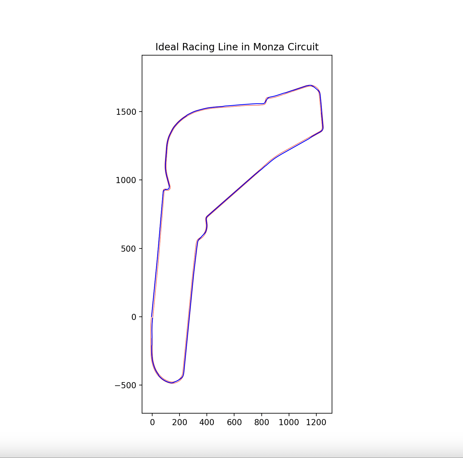
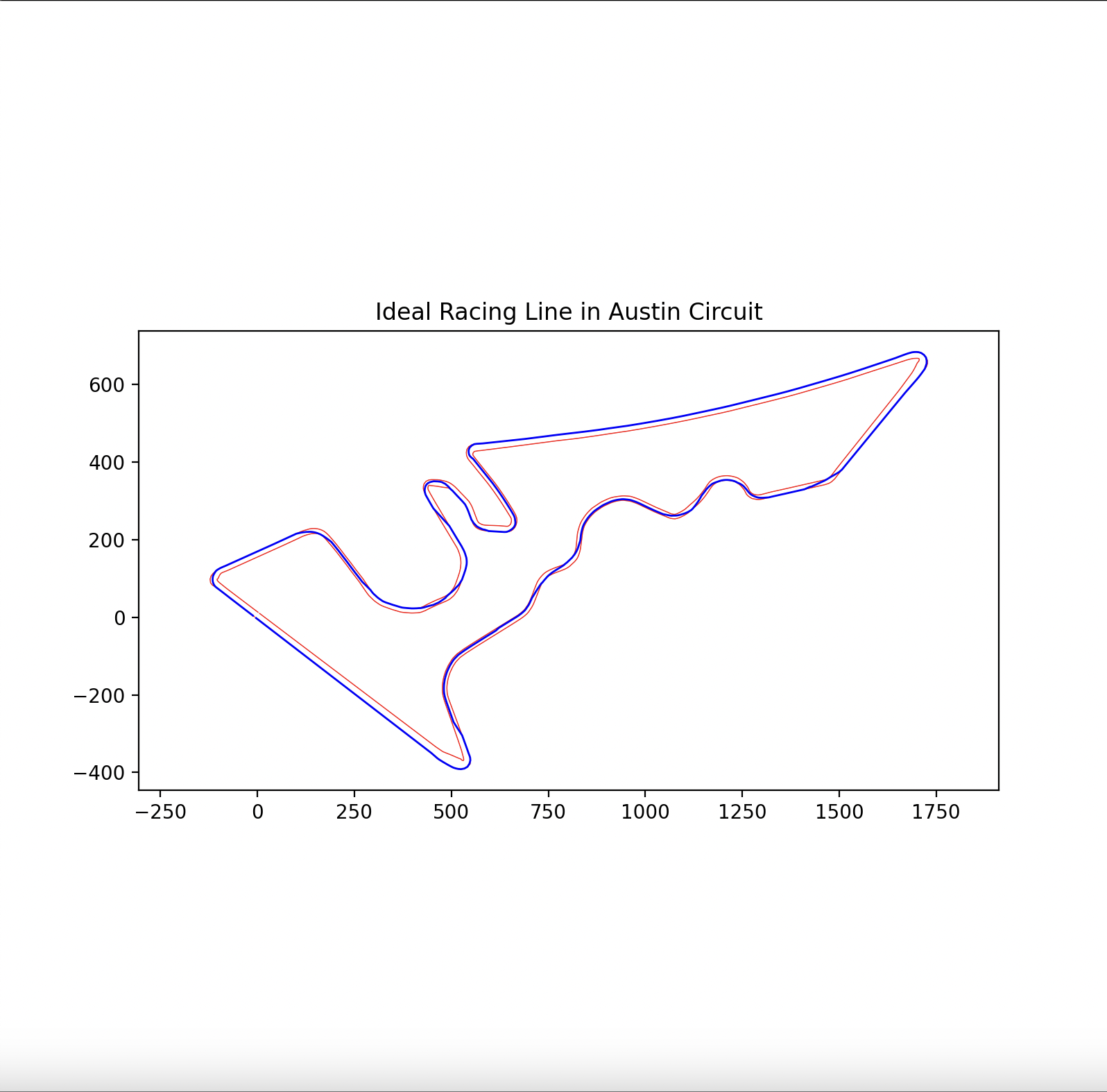
Result
Track source data is from here.
Austin Circuit
Monza Circuit